Adversarial Autoencoders

Some time ago I read an interesting paper about Adversarial Autoencoders, written by Alireza Makhzani, Jonathon Shlens, Navdeep Jaitly, and Ian Goodfellow. The idea I find most fascinating in this paper is the concept of mapping the encoder’s output distribution $q(\mathbf{z}|\mathbf{x})$ to an arbitrary prior distribution $p(\mathbf{z})$ using adversarial training (rather than variational inference).

I had some time available recently and decided to implement one myself using Lasagne and Theano. If you’re only interested in the code, it’s available on GitHub.

If you want to skip ahead, in this post we’ll provide a brief review of autoencoders, discuss adversarial autoencoders, and finally look at some interesting visualizations obtained from the resulting adversarial autoencoder.

Background

At the simplest level, an autoencoder is simply a neural network that is optimized to output the input that it is provided with, or stated alternatively, optimimized to reconstruct its input at the output layer. Typically this is implemented as two separate neural networks, namely the encoder and the decoder. The encoder takes the input and transforms it to a representation that has certain useful characteristics. The decoder, on the other hand, transforms the output of the encoder back to the original input. To avoid simply learning the identity function, certain constraints are usually placed on the output of the encoder. For example, if the dimensionality of the encoder’s output is smaller than the dimensionality of the input, the encoder is forced to compress the input in such a way that it still preserves as much of the information in the input as possible. In this case, the encoder can be used to project the data to a lower-dimensional space (similar to principal component analysis). Alternatively, we can use the Kullback-Leibler divergence to encourage the encoder’s output to resemble some prior distribution that we choose. Such autoencoders are referred to as variational autoencoders.

Autoencoders as Generative Models

We have already briefly mentioned that the properties of the encoder’s output allow us to transform input data to a useful representation. In the case of a variational autoencoder, the decoder has been trained to reconstruct the input from samples that resemble our chosen prior. Because of this, we can sample data points from this prior distribution, and feed these into the decoder to reconstruct realistic looking data points in the original data space.

Unfortunately, variational autoencoders often leave regions in the space of the prior distribution that do not map to realistic samples from the data. Adversarial autoencoders aim to improve this by encouraging the output of the encoder to fill the space of the prior distribution entirely, thereby allowing the decoder to generate realistic looking samples from any data point sampled from the prior. Instead of using variational inference, adversarial autoencoders do this by introducing two new components, namely the discriminator and the generator. These are discussed next.

Implementation of an Adversarial Autoencoder

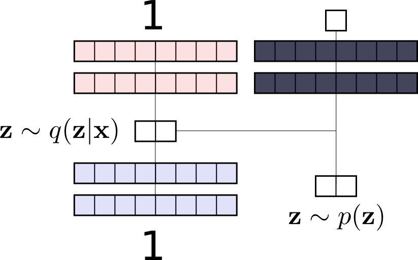
Below we demonstrate the architecture of an adversarial autoencoder. The left part of the diagram shows the encoder/decoder pair, where an input vector $\mathbf{x}$, the digit “1” in this case, is fed in as input to the encoder, transformed to the code $\mathbf{z}$ by the encoder, and then fed to the decoder that transforms it back to the original data space. On the right, a sample $\mathbf{z}$ is drawn from the prior distribution $p(\mathbf{z})$. The discriminator is optimized to separate the samples drawn from the prior distribution $p(\mathbf{z})$ from the samples drawn from the encoder distribution $q(\mathbf{z}|\mathbf{x})$.

For every minibatch, there are three important events:

1. A minibatch of input vectors is encoded and decoded by the encoder and decoder, respectively, after which both the encoder and decoder are updated based on the standard reconstruction loss.
2. A minibatch of input vectors is transformed by the encoder, after which the minibatch is concatenated with code vectors sampled from the prior distribution. The discriminator is then updated using a binary cross-entropy loss based on its ability to separate those samples generated by the encoder from those sampled from the prior distribution.
3. A minibatch of input vectors is transformed by the encoder, the source of these data points is predicted by the discriminator, and the generator (which is also the encoder) is updated using a binary cross-entropy loss based on its ability to fool the discriminator into thinking the data points came from the prior distribution.

It is interesting to note that the reconstruction loss drops fairly consistently throughout training. The adversarial losses (generative and discriminative, respectively), on the other hand, remain roughly constant after some initial fluctuation. This is the result of the adversarial training, where the discriminator’s improvement is countered by the generator’s improvement, leading to the convergence of both.

Experiments

To explore some of the properties of an adversarial autoencoder, we train it on the MNIST handwritten digit data set. The architecture we use is as described here by the author. We use two neurons in the encoder’s output layer and draw samples from a two-dimensional uniform random distribution.

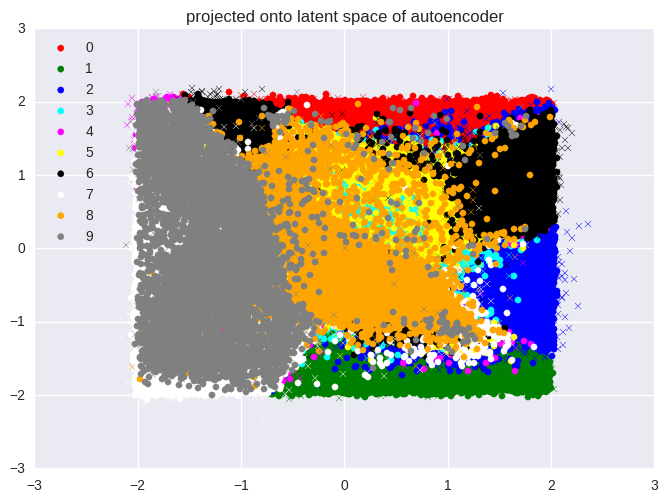
First, we show the images from the MNIST handwritten digit data set projected onto the two axes represented by the two neurons in the output of the encoder. Because we are projecting the 784-dimensional input vectors to 2-dimensional vectors, there is a lot of overlap between the classes. We clearly see, however, that practically all the data points from the training set (indicated by circles) lie within the bounds of the prior distribution. Note that some of the points from the test set (indicated by crosses) lie outside this region.

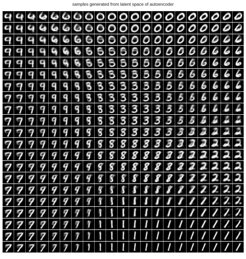
Next, we traverse the two axes of our prior distribution, sampling points from a regularly-spaced grid. For each sample, we use the decoder to generate a sample in the original data space. Note how the generated digits in each region correspond to the mapped regions of digits in the space represented by the encoder’s output.

Summary and Further Reading

We briefly discussed autoencoders and how they can be used as generative models, and then continued to describe how we can use adversarial training to impose constraints on the output distribution of the encoder. Finally, we demonstrate the ten digit classes of MNIST projected onto the encoder’s output distribution, and then traverse this space to generate realistic images in the original data space.

Those interested in further reading might want to take a look at the following links:

1. A discussion by the author on /r/machinelearning. This provides a detailed guide to implementing an adversarial autoencoder and was used extensively in my own implementation.
2. A similar post describing generative adversarial autoencoders.
3. Another implementation of an adversarial autoencoder.
4. A related paper, Deep Convolutional Generative Adversarial Networks, and the available source code.