Kaggle's Grasp and Lift EEG Detection Competition
28 Nov 2015I recently participated in Kaggle’s Grasp-and-Lift EEG Detection, as part of team Tokoloshe (Hendrik Weideman and Julienne LaChance). None of the team members had ever used deep learning for EEG data, and so we were eager to see how well techniques that are generally applied to problems in computer vision and natural language processing would generalize to this new domain. Overall, it was a fun challenge to work on and gave us a renewed appreciation for the wide range of problem domains that could potentially benefit from the incredible progress recently made in deep learning research.
Those wishing to skip ahead might be interested in the following key sections:
Background
Patients who have suffered from amputation or other neurological disabilities often have trouble performing tasks that are an essential part of everyday life. Research in devices like brain-computer interfaces aims to provide these people with prosthetic limbs that may be controlled by means of an interface to the brain. Ideally, this would enable these people to regain abilities that are often taken for granted, thereby providing them with greater mobility or independence.
Problem Statement
The goal of the challenge is to predict when a hand is performing each of six different actions given electroencephalography (EEG) signals. The EEG signals are obtained from sensors placed on a subject’s head, and the subject is then instructed to perform each of the six actions in sequence.
The Data
We are provided with EEG signals for 12 different subjects, each consisting of 10 series of trials. Each series consists of a variable number of trials, but typically around 30. One trial is defined as the progressive sequence of actions from the first to the sixth action. The six actions that we wish to predict are
- HandStart
- FirstDigitTouch
- BothStartLoadPhase
- LiftOff
- Replace
- BothReleased
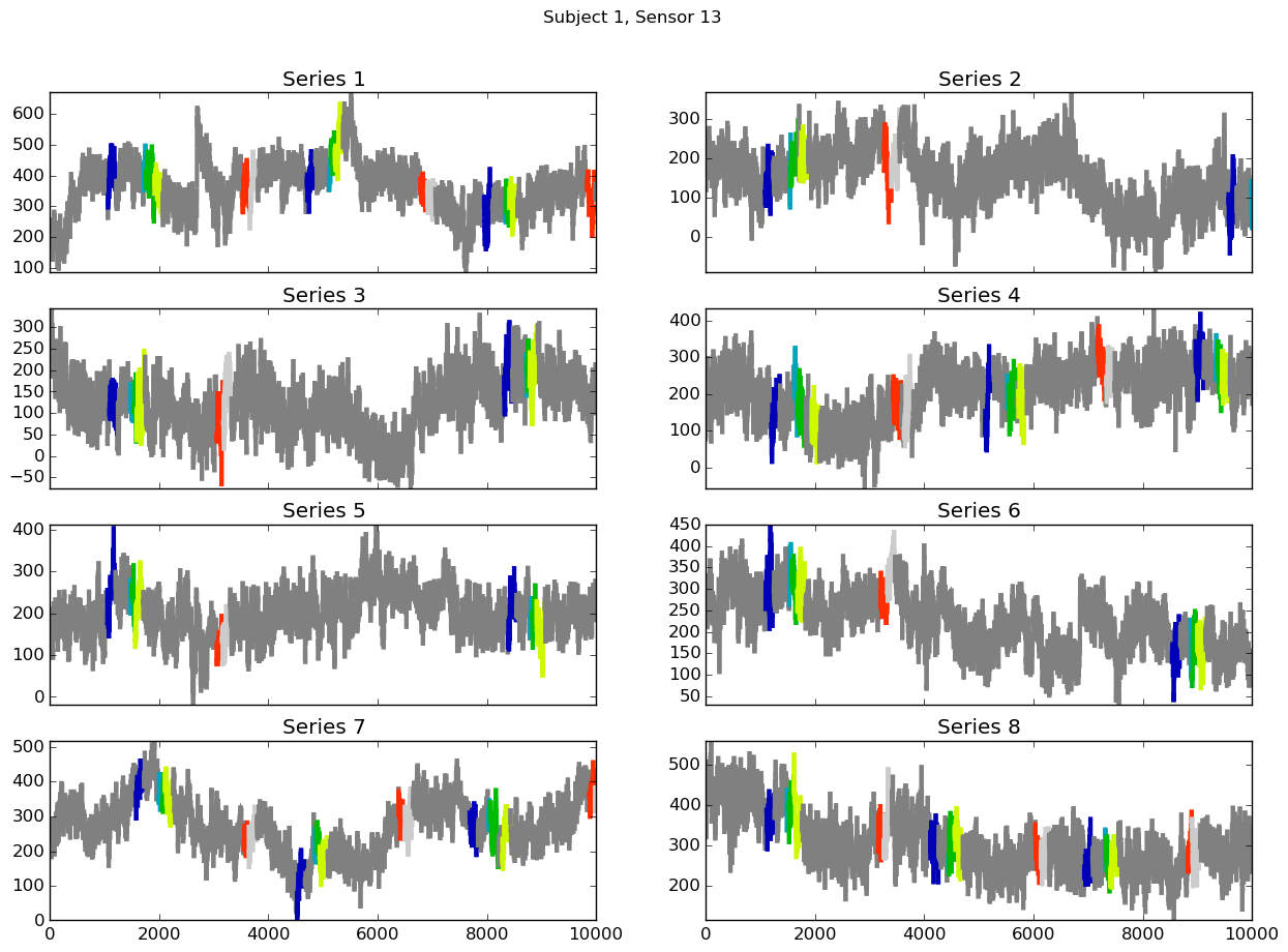
In particular, the EEG signal for each trial consists of a real value for each of the 32 channels at every time step in the signal. The subject’s EEG responses are sampled at 500 Hz, and so the time steps are 2ms from each other. For each time step, we are provided with six labels, describing which of the six actions are active at that time step. Note that an action is labeled as active if it occurred within 150ms of the current time step (future or past). The implication of this is that multiple actions may be labeled as active simultaneously. Below we show the eight series from sensor 13 for subject 1 provided for training. The colors indicate the different actions, gray indicates that no action is active. Note the amount of variation between the signals, even for a single sensor and a single subject.
Because we are working with time data, it is critical to note that we are not allowed to use data from the future when making predictions. It is simpler to think of this in terms of the practical usage of such a system - when predicting the action that a user is performing, the system will not have access to EEG signal responses that have not occurred yet. In practice, this means that we are free to train on any of the training data that we want. However, when we make a prediction for a particular time step in the test set, we may only use EEG responses from time steps that occurred at or before that time step. This is important to keep in mind, because we are provided with the EEG responses for all time steps in the test set. Care should be taken that these are in no way used when making submissions to the competition (such as when centering or scaling the signals).
More detailed information about the data may be found on Kaggle or in the original paper, Multi-channel EEG recordings during 3,936 grasp and lift trials with varying weight and friction.
Challenges
As with all machine learning problems, there are some challenges with this data set. Primarily, EEG signals are notoriously noisy, and we are given 32 channels, several of which likely do not correlate well with which of the actions are active. Additionally, the signals vary considerably from person to person and even series to series.
Our Team’s Solution
Given that our primary goal of participating in this challenge was to explore a new problem domain using deep learning, we wanted to build a system that is neither subject nor action-specific. Thus, our system is trained to predict actions given EEG signals, with no regard for which person or action it is working with. We also experimented with subject-specific models, but achieved worse performance. We suspect that the additional data from other subjects helps to regularlize the very large capacity of our deep learning models, thereby improving generalization across all subjects and actions.
Data Preparation
To build our training set, we chunk the EEG signals into fixed length sequences, that we refer to as time windows. We label each time window with six binary values indicating which of the six actions are active at the time step corresponding to the last time step in the time window. To normalize the data, we subtract the mean computed over all series from all subjects, and divide by the standard deviation computed similarly. For validation data, we keep two series from each subject separate and train on the remaining six. We do this so that we can monitor that our model is not fitting certain subjects while neglecting others.
System Architecture
Below we describe the implementation of our solution.
Deep Convolutional Neural Network
Our deep convolutional neural network has eight one-dimensional convolutional layers, four max-pooling layers, and three dense layers. The final dense layer has six output neurons, each with a sigmoid activation function that predicts the probability that a given action is active. We use the rectified linear unit (ReLU) as the activation function in all layers except for the output layer. Dropout with p = 0.5 is applied in the first two dense layers.
Input
We use time windows of 2000 time steps, that is, each time window observes four seconds of EEG signal. As described below, we subsample this time window so that only 200 time steps are actually used when feeding the example to the deep convolutional neural network.
Loss
Because the challenge’s evaluation metric, the mean column-wise area under the ROC curve, is not differentiable, we instead minimize the binary cross-entropy loss, taking the mean across the loss for each of the six actions. Even though these two are not exactly equivalent, minimizing this loss function should generally lead to better performance on the challenge’s evaluation metric.
Implementation
Our solution uses Lasagne and Theano for the implementation of the convolutional neural network. We also use scikit-learn, pandas, and matplotlib for various utilities. We developed our solution using Ubuntu 15.04. The code is available on GitHub.
Hardware
We trained our deep convolutional neural network on a computer with an NVIDIA Quadro K4200 and 16GB of RAM.
Performance Tricks
While designing our model, there were a few simple tricks that we came up with that improved our model’s performance on the held-out validation data. These are briefly described below.
Subsampling Layer
When feeding each time window into the deep convolutional neural network, we first subsample every Nth point. Not only does this greatly reduce the computational burden, but it also helps to reduce overfitting. Our initial idea was to use this as a form of data augmentation, where we would sample every Nth point starting from different time steps in the time window, but this did not seem have any effect.
Window Normalization Layer
We found that normalizing the values in each time window to be between 0 and 1 greatly improved generalization. This was done by simply using the minimum and maximum values in each time window to compute a transformation to the desired range. We suspect that this is because the relative difference between points in the time window is more important than the actual amplitudes, and so by normalizing for this difference we encourage the model to fit the actual signal, rather than the noise.
Results
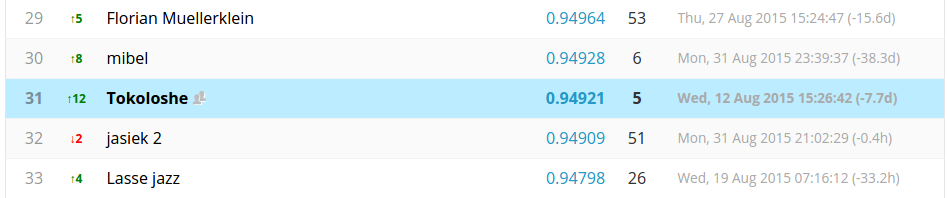
Our final solution earned us a spot in the Top 10% on the challenge’s
private leaderboard.
Other Ideas
Throughout this challenge, we had numerous other ideas that we could never quite get to work. One in particular was the concept of data augmentation, which is the generation of more training examples by transforming existing training examples in such a way that the relationship to the corresponding label is preserved. There were two key ideas that we tried, namely
- subsample each time window from a random starting position, so that the network only occasionally sees the exact time window twice, and
- increase the number of positive training examples (training examples where an action is active) by duplicating existing training examples, where each duplicated example gets a small amount of Gaussian noise added to it.
Unfortunately, neither of these ideas enabled our model to generalize better to unseen test data.
Final Words
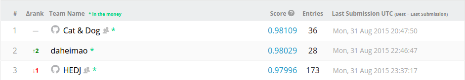
We are very excited to see the scores achieved on the challenge’s leaderboard, as this certainly indicates that deep learning has the potential to contribute to further progress in the field of brain-computer interfaces and the analysis of EEG signals. We would also like to congratulate the top three teams:
Anyone interested in their solutions may follow the above links to their own descriptions of their solutions. Finally, we would also like to give special thanks to Alexandre Barachant from team Cat & Dog, for publicly sharing so much of his knowledge related to brain-computer interfaces and EEG signals.