Orthogonal Initialization in Convolutional Layers

12 Dec 2015

In Exact solutions to the nonlinear dynamics of learning in deep linear neural networks Saxe, McClelland, and Ganguli investigate the question of how to initialize the weights in deep neural networks by studying the learning dynamics of deep linear neural networks. In particular, they suggest that the weight matrix should be chosen as a random orthogonal matrix, i.e., a square matrix $W$ for which $W^TW = I$.

In practice, initializing the weight matrix of a dense layer to a random orthogonal matrix is fairly straightforward. For the convolutional layer, where the weight matrix isn’t strictly a matrix, we need to think more carefully about what this means.

In this post we briefly describe some properties of orthogonal matrices that make them useful for training deep networks, before discussing how this can be realized in the convolutional layers in a deep convolutional neural network.

Introduction

Two properties of orthogonal matrices that are useful for training deep neural networks are

they are norm-preserving, i.e., $||Wx||_2 = ||x||_2$, and
their columns (and rows) are all orthonormal to one another, i.e., $w_{i}^Tw_{j} = \delta_{ij}$, where $w_{i}$ refers to the $i$th column of $W$.

At least at the start of training, the first of these should help to keep the norm of the input constant throughout the network, which can help with the problem of exploding/vanishing gradients. Similarly, an intuitive understanding of the second is that having orthonormal weight vectors encourages the weights to learn different input features.

Dense Layers

Before we discuss how the orthogonal weight matrix should be chosen in the convolutional layers, we first revisit the concept of dense layers in neural networks. Each dense layer contains a fixed number of neurons. To keep things simple, we assume that the two layers $l$ and $l+1$ each have $m$ neurons. Let $W$ be an $m \times m$ matrix where the $i$th row contains the weights incoming to neuron $i$ in layer $l+1$, $\mathbf{x}$ be a $m \times 1$ vector containing the $m$ outputs from the neurons in layer $l$, and $\mathbf{b}$ be the vector of biases. Then we can describe the pre-activation of layer $l+1$ as $\mathbf{z}$,

$\mathbf{z} = \left[ \begin{matrix} w_{11} & w_{12} & \cdots & w_{1m} \\ w_{21} & w_{22} & \cdots & w_{2m} \\ \vdots & \vdots & \ddots & \vdots \\ w_{m1} & w_{m2} & \cdots & w_{mm} \\ \end{matrix} \right] \left[ \begin{matrix} x_{1} \\ x_{2} \\ \vdots \\ x_{m} \\ \end{matrix} \right] + \left[ \begin{matrix} b_{1} \\ b_{2} \\ \vdots \\ b_{m} \\ \end{matrix} \right],$

where the activation function $f(\mathbf{z})$ is applied to produce the final output of layer $l+1$. In the following figure we show how the outputs from the previous layer, $x_1, \ldots, x_j, \ldots, x_m$, are multiplied by the $i$th neuron’s weights, $w_1, \ldots, w_j, \ldots, w_m$, the bias is added, and the activation function applied.

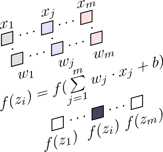
In this formulation, the idea behind orthogonal initialization is to choose the weight vectors associated with the neurons in layer $l+1$ to be orthogonal to each other. In other words, we want the rows of $W$ to be orthogonal to each other.

Convolutional Layers

In a convolutional layer, each neuron is sparsely connected to several small groups of neurons in the previous layer. Even though each convolutional kernel is technically a $k \times k$ matrix, in practice the convolution can be thought of as an inner product between two $k^2$-dimensional vectors, i.e., $\mathbf{x} \ast \mathbf{w} = \sum\limits_{i=1}^{k^2}x_i \cdot w_i$.

Below we show how a different convolutional kernel is applied to each channel in layer $l$, the results summed, the bias added, and the activation function applied.

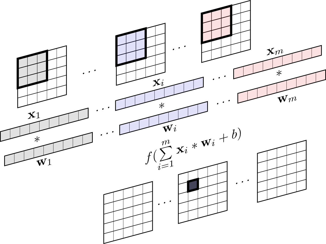
Now it becomes clear that we should choose each channel in layer $l+1$ to have a “weight vector” that is orthogonal to the weight vectors of the other channels. When we say “weight vector” in the convolutional layer, we really mean the kernel-as-vector for each of the channels stacked next to each other. This is similar to how it was done in the dense layer, but now the weight vector is no longer connected to every neuron in layer $l$.

Implementation

We can check this intuition by examining how the orthogonal weight initialization is implemented in a popular neural network library such as Lasagne. Suppose we want a matrix with $m$ rows, with $m$ the number of channels in layer $l+1$, where the rows are all orthogonal to one another. Each row is a vector of dimension $nk^2$, where $n$ is the number of channels in layer $l$, and $k$ is the dimension of the convolutional kernel. For practical purposes, let us choose $m = 64$, $n = 32$, and $k = 3$, i.e., layer $l + 1$ has $64$ channels, each learning a $3 \times 3$ kernel for each of the $32$ channels in layer $l$.

Similar to how it’s implemented in Lasagne, we can use the Singular Value Decomposition (SVD). Given a random matrix $X$, we compute the reduced SVD, $X = \hat{U}\hat{\Sigma}\hat{V}^T$, and then use the rows of the matrix $V^T$ as our orthogonal weight vectors (in this case the weight vectors are also orthonormal). So, in Python:

>>> import numpy as np
>>> X = np.random.random((64, 32 * 3 * 3))
>>> U, _, Vt = np.linalg.svd(X, full_matrices=False)
>>> Vt.shape
(64, 288)
>>> np.allclose(np.dot(Vt, Vt.T), np.eye(Vt.shape[0]))
True
>>> W = Vt.reshape((64, 32, 3, 3))

Finally, we can use the matrix $W$ to initialize the weights of the convolutional layer. Keep in mind, however, that in practice the elements of $W$ are often scaled to compensate for the change in norm brought about by the activation function.

Conclusion

Orthogonal initialization has shown to provide numerous benefits for training deep neural networks. It is easy to see which vectors should be orthogonal to one another in a dense layer, but less straightforward to see where this orthogonality should happen in a convolutional layer, because the weight matrix is no longer really a matrix. By considering that neurons in a convolutional layer serve exactly the same purpose as neurons in a dense layer but with sparse connectivity, the analogy becomes clear.

Hendrik J. Weideman