Quantifying Uncertainty in Neural Networks

As part of my research on applying deep learning to problems in computer vision, I am trying to help plankton researchers accelerate the annotation of large data sets. In terms of the actual classification of plankton images, excellent progress has been made recently, largely thanks to the popular 2015 Kaggle National Data Science Bowl. In this competition, the goal was to predict the probability distribution function over 121 different classes of plankton, given a grayscale image containing a single plankton organism. The winning team’s solution is of particular interest, and the code is available on GitHub.

While this progress is encouraging, there are challenges that arise when using deep convolutional neural networks to annotate plankton data sets in practice. In particular, unlike in most data science competitions, the plankton species that researchers wish to label are not fixed. Even in a single lake, the relevant species may change as they are influenced by seasonal and environmental changes. Additionally, because of the difficulties involved in collecting high-quality images of plankton, a large training set is often unavailable.

For the reasons given above, for any system to be practically useful, it has to

1. recognize when an image presented for classification contains a species that was absent during training,

2. acquire the labels for the new class from the user, and

3. extend its classification capabilities to include this new class.

In this post, we consider the first point above, i.e., how we can quantify the uncertainty in a deep convolutional neural network. A brief overview with links to the relevant sections is given below.

1. Background: why interpreting softmax output as confidence scores is insufficient.
2. Bayesian Neural Networks: we look at a recent blog post by Yarin Gal that attempts to discover What My Deep Model Doesn’t Know…
3. Experiments: we attempt to quantify uncertainty in a model trained on CIFAR-10.
4. Code: all the code is available on GitHub.

Background

Although it may be tempting to interpret the values given by the final softmax layer of a convolutional neural network as confidence scores, we need to be careful not to read too much into this. For example, consider that recent work on adversarial examples has shown that imperceptible perturbations to a real image can change a deep network’s softmax output to arbitrary values. This is especially important to keep in mind when we are dealing with images from classes that were not present during training. In Deep Neural Networks are Easily Fooled: High Confidence Predictions for Unrecognizable Images, the authors explain how the region corresponding to a particular class may be much larger than the space in that region occupied by training examples from that class. The result of this is that an image may lie within the region assigned to a class and so be classified with a large peak in the softmax output, while still being far from images that occur naturally in that class in the training set.

Bayesian Neural Networks

In an excellent blog post, Yarin Gal explains how we can use dropout in a deep convolutional neural network to get uncertainty information from the model’s predictions. In a Bayesian neural network, instead of having fixed weights, each weight is drawn from some distribution. By applying dropout to all the weight layers in a neural network, we are essentially drawing each weight from a Bernoulli distribution. In practice, this mean that we can sample from the distribution by running several forward passes through the network. This is referred to as Monte Carlo dropout.

Experiments

Quantifying the uncertainty in a deep convolutional neural network’s predictions as described in the blog post mentioned above would allow us to find images for which the network is unsure of its prediction. Ideally, when given a new unlabeled data set, we could use this to find images that belong to classes that were not present during training.

To investigate this, we train a deep convolutional neural network similar to the one used in Bayesian Convolutional Neural Networks with Bernoulli Approximate Variational Inference and as described on GitHub. The goal was to train this network on the ten classes of CIFAR-10, and then evaluate the certainty of its predictions on classes from CIFAR-100 that are not present in CIFAR-10.

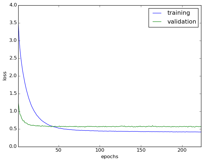
We train the model on the 50000 training images and used the 10000 test images provided in CIFAR-10 for validation. All parameters are the same as in the implementation provided with the paper, namely a batch size of 128, weight decay of 0.0005, and dropout applied in all layers with $p = 0.5$. The learning rate is initially set to $l = 0.01$, and is updated according to $l_{i+1} = l_{i} (1 + \gamma i)^{-p}$, with $\gamma = 0.0001$ and $p = 0.75$, after the $i$th weight update. The learning curve is shown below. The best validation loss is 0.547969 and the corresponding training loss is 0.454744.

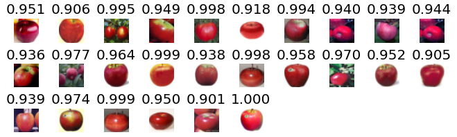
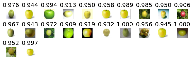
Now that we have a deep convolutional network trained on the ten classes of CIFAR-10, we present images from the apple class from CIFAR-100 to the network. We run $T=50$ stochastic forward passes through the network and take the predictive mean of the softmax output. The results, while a little discouraging, are amusing. It seems that the network is very happy to classify red apples as automobiles, and green apples as frogs with low uncertainty. Below we show apples that were classified as automobiles with $p > 0.9$, and then similarly for frogs. The number above each image is the maximum of the softmax output, computed as the mean of the 50 stochastic forward passes.

Code

All of the code used in the above experiment is available on GitHub. The non-standard dependencies are Lasagne, Theano, OpenCV (for image I/O), and Matplotlib.

Discussion

It is clear that the convolutional neural network has trouble with images that appear at least somewhat visually similar to images from classes that it saw during training. Why these misclassifications are made with low uncertainty requires further investigation. Some possibilities are mentioned below.

1. With only ten classes in CIFAR-10, it is possible that the network does not need to learn highly discriminative features to separate the classes, thereby causing the appearance of these features in another class to lead to a high-confidence output.

2. The saturating softmax output leads to the same output for two distinct classes (one present and one absent during training), even if the input to the softmax is very different for the two classes.

3. The implementation of a Bayesian neural network with Monte Carlo dropout is too crude of an approximation to accurately capture the uncertainty information when dealing with image data.

Conclusion

To build a tool that can be used by plankton researchers to perform rapid annotation of large plankton data sets, we need to quantify the uncertainty in a deep learning model’s predictions to find images from species that were not present during training. We can capture this uncertainty information with a Bayesian neural network, where dropout is used in all weight layers to represent weights drawn from a Bernoulli distribution. A quick experiment to classify a class from CIFAR-100 using a model trained only on the classes from CIFAR-10 shows that this is not trivial to achieve in practice.

Hopefully we shall be able to shed some light on the situation and address some of these problems as the topic of modeling uncertainty in deep convolutional neural networks is explored more in the literature.