Semi-Supervised Learning with DCGANs

I recently wanted to try semi-supervised learning on a research problem. In Improved Techniques for Training GANs the authors show how a deep convolutional generative adversarial network, originally intended for unsupervised learning, may be adapted for semi-supervised learning. It wasn’t immediately clear to me how the equations in Section 5 of the paper are equivalent to OpenAI’s implementation, so I decided to go through the derivation myself. In this post, I’ll show how the supervised and unsupervised loss functions in the implementation may be derived from the equations provided in the paper. If you’re already familiar with the background, skip ahead to the supervised loss or unsupervised loss derivation.

I’ve previously written about adversarial learning and others have written several good posts about semi-supervised learning with deep convolutional generative adversarial networks (DCGANs), so it would be superfluous for me to cover the architecture and optimization. Thus, I’ll only provide enough background necessary to understand the loss function. Those interested in a more thorough discussion with TensorFlow code might want to read Thalles Silva’s blog post, Semi-supervised learning with Generative Adversarial Networks (GANs).

Background

Unlike supervised learning, where we have labels for all training examples, and unsupervised learning, where we don’t have any labels at all, in semi-supervised learning we have labels for some, but not all, training examples. Clearly, we should extract any useful information that is available from the unlabeled examples, even if we don’t know their labels explicitly. Thus, training a semi-supervised DCGAN for classification consists has four parts, namely

1. the discriminator must predict the correct label for those training examples with labels (exactly like supervised learning),
2. the discriminator must verify that the unlabeled training examples were drawn from the original data distribution, i.e., belong to one of the known classes even if we don’t know which one,
3. the discriminator must claim that samples drawn from the generator are fake, i.e., do not belong to one of the known classes, and finally,
4. the generator must continually improve its fake samples to fool the discriminator into thinking that they are real.

Taken together, the idea is that the discriminator acts as a conventional multi-class classifier, while simultaneously learning to map the unlabeled training examples to the same feature distribution.

Deriving the Loss Functions

To realize the four points described above with a differentiable loss function, the authors of Improved Techniques for Training GANs propose using a $K+1$-class classifier, where the first $K$ outputs correspond to the probabilities of the $K$ classes. Effectively, this means that the sum over the first $K$ outputs may be interpreted as the probability that the given example is real, and the output at $K+1$ as the probability that the example is fake. They note, however, that such a classifier is over-parameterized. This is analogous to how a binary classifier requires only a single output neuron to produce the probabilities of the two classes. Thus, the same result may be achieved using a $K$-class classifier as the discriminator. Although the derivation is straightforward, it’s easy to see this with a small code example:

# Not a numerically stable implementation of softmax, just as an example.
>>> def softmax(x):
>>>    return np.exp(x) / np.sum(np.exp(x))
>>> x = np.random.random(8)
# Probabilities do not change if we shift them such that final logit is 0.
>>> np.allclose(softmax(x), softmax(x - x[-1]))
True

Supervised Loss

With a $K$-class classifier, the supervised loss simply becomes the categorical cross-entropy loss. Let $\mathbf{x} \in [-1, 1]^{H \times W \times 3}$ be a single training example (an RGB-image normalized to the same range as the generator’s output) and $\mathbf{y} \in \{0, 1\}^{K} \mid \sum\limits_{i=1}^{K}y_i = 1$ (a one-hot vector indicating to which class $\mathbf{x}$ belongs). The discriminator takes the input $\mathbf{x}$ and produces the $K$-dimensional vector of logits $l(\mathbf{x})$ at the final layer. The predicted probability $\hat{y}_j$ for class $j$ is computed using the softmax function

which we substitute into the categorical cross-entropy loss

Because $\mathbf{y}$ is a one-hot vector, we know that it is zero everywhere except for the index representing the class to which $\mathbf{x}$ belongs. Let this index be $j’$, such that $y_i = 0 \quad\forall_{i \neq j’}$ and $y_{j’} = 1$. All terms in the outer summation become zero except for $j = j’$, and so the loss function may be simplified to

After taking the average over all training examples in the minibatch, this gives us the supervised loss function provided in the implementation.

l_lab = output_before_softmax_lab[T.arange(args.batch_size),labels]
loss_lab = -T.mean(l_lab) + T.mean(T.mean(nn.log_sum_exp(output_before_softmax_lab)))

Unsupervised Loss

Because we’re simply going to average the loss over the minibatch anyway, we compute the loss for a single example to keep things simple. Let $\mathbf{x}_{real} \in [-1, 1]^{H \times W \times 3}$ be a single training example (for which we don’t know the label) and $\mathbf{x}_{fake} \in [-1, 1]^{H \times W \times 3}$ be a single example sampled from the generator. For the unsupervised loss, the discriminator must maximize the log-probability that $\mathbf{x}_{real}$ is real and minimize the log-probability that $\mathbf{x}_{fake}$ is real,

where $D(\mathbf{x})$ is simply the softmax over the $K$ logits and a dummy logit fixed to $l_{k+1}(\mathbf{x}) = 0$ that appears as $e^0 = 1$ in the denominator to represent the “fake” class, i.e.,

where

is the sum of the exponents of the logits representing the “real” classes. Substituting and simplifying, we get

Noting that $\log\left(\sum\limits_{k=1}^{K}e^{l_k(\mathbf{x})} + 1\right) = \text{Softplus}\left(\log\sum\limits_{k=1}^{K}e^{l_k(\mathbf{x})}\right)$, we get

After averaging each term over all examples in the minibatch and scaling by $0.5$ to account for the fact that we have effectively doubled the batch size relative to the supervised loss, we get the unsupervised loss defined in the implementation.

l_unl = nn.log_sum_exp(output_before_softmax_unl)
l_gen = nn.log_sum_exp(output_before_softmax_gen)
loss_unl = -0.5*T.mean(l_unl) + 0.5*T.mean(T.nnet.softplus(l_unl)) + 0.5*T.mean(T.nnet.softplus(l_gen))

Conclusion

Initially developed for unsupervised representation learning, deep convolutional generative adversarial networks have been shown also to be effective for semi-supervised learning. Although the combination of supervised and unsupervised losses presented in Section 5 of Improved Techniques for Training GANs may initially seem not to resemble those in the official implementation, careful derivation makes the equivalence clear.

References

1. Unsupervised Representation Learning with Deep Convolutional Generative Adversarial Networks
2. Improved Techniques for Training GANs
3. Semi-supervised learning with Generative Adversarial Networks (GANs)

Piping the Output of a Command to the Clipboard

This is a simple post about how to pipe the output of a command to the clipboard on Ubuntu, i.e., a way to get the output of a command such as

readlink -f 2007_000027.jpg  # gets the canonical path

to the clipboard without using the mouse. If you just want the command, skip ahead to the bash alias.

The Problem

When designing computer vision (and other) algorithms, one often encounters strange edge cases — situations where an algorithm that has successfully processed thousands of images fails spectacularly on one particular input. Generally, a quick check of the problem image in an image viewer like feh or an interactive shell like IPython can identify some of the more common bugs (corrupted image data, integer overflow/underflow, etc.).

Getting a specific image into IPython, for example, requires first selecting the filepath with the mouse (drag-select or double-click), copying with Ctrl-Shift-C, and then loading it with something like:

img = cv2.imread('<Ctrl-Shift-V here>')

Without starting a flame war (Is using a mouse less efficient?), I find the keyboard to be significantly faster than the mouse for frequently-used commands in a keyboard-friendly environment, like vim and i3. As a result, I want to achieve the above without using the mouse.

The Solution

A quick Google search reveals that xclip is a good place to start. A good idea, however, is first to strip any trailing newline from the input to ensure that it is not interpreted as a command. Thus, the full command becomes

readlink -f 2007_000027.jpg | xargs echo -n | xclip -selection clipboard

This gets the canonical path to the file 2007_000027.jpg, strips the trailing newline, and sends the result to the clipboard.

As a Bash Alias

We can make this more convenient by adding the following line to ~/.bash_aliases:

alias xclip='xargs echo -n | xclip -selection clipboard'

Now, we can easily load a given image by simply piping its canonical path to the clipboard. For example,

readlink -f 2007_000027.jpg | xclip

gets us

/media/hdd/hendrik/datasets/pascal-2011/TrainVal/VOCdevkit/VOC2011/JPEGImages/2007_000027.jpg

with Ctrl-Shift-V. No mouse involved.

Training a char-rnn to Talk Like Me

Someone recently suggested to me the possibility of training a char-rnn on the entire history of my Facebook conversations. The idea would be to see if the result sounds anything like me. When I first started out, my idea was simply to use one of the existing char-rnn implementations, for example this one written using Torch, or this one, written using Lasagne and Theano. Along the way, however, I decided that it would be a good learning experience to implement a char-rnn myself. If you’re only interested in the code, it’s available on Github.

As a result, this post now consists of two parts. The first provides a very brief overview of how a char-rnn works. I keep it brief because others have already done excellent work to provide extensive insights into the details of a char-rnn, for example, see this blog post by Andrej Karpathy. The second describes how I trained this char-rnn on my own Facebook conversations, and some of the things I discovered.

Background of char-rnn

In this section, I’ll provide a very brief overview of how a char-rnn works. If you’re interested in an extensive discussion instead, I recommend that you rather read the blog post mentioned above.

The term “char-rnn” is short for “character recurrent neural network”, and is effectively a recurrent neural network trained to predict the next character given a sequence of previous characters. In this way, we can think of a char-rnn as a classification model. In the same way that we output a probability distribution over classes when doing image classification, for a char-rnn we wish to output a probability distribution over character classes, i.e., a vocabulary of characters. 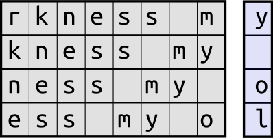Unlike image classification where we are given a single image and expected to predict an output immediately, however, in this setting we are given the characters one at a time and only expected to predict an output after the last character. This is illustrated below. Consider the sequence of characters, “Hello darkness my old friend”, where the sequence of characters marked in bold are observed by the model. At each step, the model observes a sequence of eight characters (show on the left) and is asked to predict the next one (on the right).

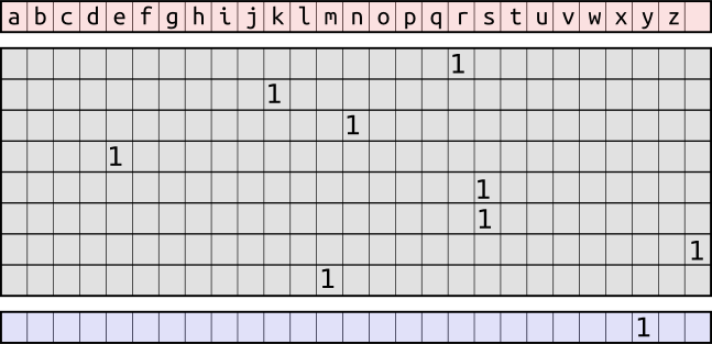
In practice, each character is typically encoded as a one-hot vector, where the position of the one indicates the position of the character in the vocabulary. For example, in a vocabulary consisting of the twenty-six lower-case letters and space, the first row of the sequence above would be encoded as demonstrated in the figure below. Note that zeros are represented by empty cells to reduce clutter. The top row shows the characters in the vocabulary, the grid shows each character in the sequence converted to its one-hot representation, and the bottom row shows the target character’s one-hot representation.

Because this is effectively a classification task, where the output classes are characters in the vocabulary, we use the standard categorical cross-entropy loss to train the model. If we let $\mathbf{y}$ be a vector representing the one-hot encoding of the target character and $\mathbf{\hat{y}}$ the vector of probabilities over the $n$ characters in the vocabulary as produced by the output layer of the char-rnn, then the loss for a single target character is defined as $-\sum\limits_{i=1}^{n}y_i\log(\hat{y}_i)$.

By iteratively minimizing this loss, we obtain a model that predicts characters consistent with the sequences observed during training. Note that this is a fairly challenging task, because the model starts with no prior knowledge of the language being used. Ideally, this model would also capture the style of the author, which we explore next.

Training a char-rnn on my Facebook Conversations

After implementing a char-rnn as described above, I decided to train it on the entire history of my Facebook conversations. To do this, I first downloaded my chat history. This can be achieved by clicking on “Privacy Shortcuts”, “See More Settings”, “General”, and finally “Download a copy of your Facebook data”. These instructions are available here.

Next, clone this Facebook chat parser and install it:

git clone https://github.com/ownaginatious/fbchat-archive-parser
python setup.py develop

Now unzip the downloaded archive and parse it. The filepath should point to the messages.htm file inside the unzipped archive.

fbcap html/messages.htm > messages.txt

At this point, you have a text file messages.txt containing the data, sender, and text of every message from your Facebook conversation history. To train the char-rnn, however, I wanted to train only on messages written by me. To do this, I used the this code snippet to parse out messages indicating me as the sender. You can use this snippet too, or write your own, more sophisticated parser if you want more control over which messages to use for the training data.

Finally, set the text_fpath variable in the train_char_rnn.py file, and run python train_char_rnn.py. At first, the output will be mostly gibberish, with alternating short words repeated for the entire sequence. I started seeing somewhat more intelligible output after about twelve hours of training on an NVIDIA TITAN X.

Results

After training the model on the entire history of my Facebook conversations, we can generate sequences from the model by feeding an initial sequence and then repeatedly sampling from the model. This can be done by using the generate_samples.py file. Set the text_fpath to the same text file used to train the model (to build the vocabulary), and run python generate_samples.py.

Next, we show some samples from the model. The phrase used to initialize the model is shown in italics.

1. The meaning of life is to find them? Oh, I don’t know if I would be able to publish a paper on that be climbing today, but it will definitely know what that makes sense. I’m sure they wanted to socialis that I am bringing or

2. What a cruel twist of fate, that we should be persuate that 😂 And cook :D I will think that’s mean I think I need to go to the phoebe? That’s awesome though Haha, sorry, I don’t know if it was more time to clas for it’s badass though I jus

3. The fact of the matter is just the world to invite your stuff? I don’t know how to right it wouldn’t be as offriving for anything, so that would be awesome, thanks :) I have no idea… She would get to worry about it :P And I

4. At the very least, you should remember that as a house of a perfect problems 😂 Yeah :D I wonder how perfect for this trank though So it’s probably foltower before the bathers will be fine and haven’t want to make it worse Thanks for one of

Looking at these samples, it would appear as if the model has learned decent spelling and punctuation, but struggles to formulate sensible sentences. I suspect that the training data was too limited, as the entire text file is only about 1.5MB. Additionally, unlike email, Facebook messages often consist of short replies rather than multiple, full sentences. At the end of the day, I highly doubt I could fool anyone by having the char-rnn auto-reply to them. On the other hand, I don’t think releasing a model that’s been trained on every message I’ve ever sent would be a good idea either.

Adversarial Autoencoders

Some time ago I read an interesting paper about Adversarial Autoencoders, written by Alireza Makhzani, Jonathon Shlens, Navdeep Jaitly, and Ian Goodfellow. The idea I find most fascinating in this paper is the concept of mapping the encoder’s output distribution $q(\mathbf{z}|\mathbf{x})$ to an arbitrary prior distribution $p(\mathbf{z})$ using adversarial training (rather than variational inference).

I had some time available recently and decided to implement one myself using Lasagne and Theano. If you’re only interested in the code, it’s available on GitHub.

If you want to skip ahead, in this post we’ll provide a brief review of autoencoders, discuss adversarial autoencoders, and finally look at some interesting visualizations obtained from the resulting adversarial autoencoder.

Background

At the simplest level, an autoencoder is simply a neural network that is optimized to output the input that it is provided with, or stated alternatively, optimimized to reconstruct its input at the output layer. Typically this is implemented as two separate neural networks, namely the encoder and the decoder. The encoder takes the input and transforms it to a representation that has certain useful characteristics. The decoder, on the other hand, transforms the output of the encoder back to the original input. To avoid simply learning the identity function, certain constraints are usually placed on the output of the encoder. For example, if the dimensionality of the encoder’s output is smaller than the dimensionality of the input, the encoder is forced to compress the input in such a way that it still preserves as much of the information in the input as possible. In this case, the encoder can be used to project the data to a lower-dimensional space (similar to principal component analysis). Alternatively, we can use the Kullback-Leibler divergence to encourage the encoder’s output to resemble some prior distribution that we choose. Such autoencoders are referred to as variational autoencoders.

Autoencoders as Generative Models

We have already briefly mentioned that the properties of the encoder’s output allow us to transform input data to a useful representation. In the case of a variational autoencoder, the decoder has been trained to reconstruct the input from samples that resemble our chosen prior. Because of this, we can sample data points from this prior distribution, and feed these into the decoder to reconstruct realistic looking data points in the original data space.

Unfortunately, variational autoencoders often leave regions in the space of the prior distribution that do not map to realistic samples from the data. Adversarial autoencoders aim to improve this by encouraging the output of the encoder to fill the space of the prior distribution entirely, thereby allowing the decoder to generate realistic looking samples from any data point sampled from the prior. Instead of using variational inference, adversarial autoencoders do this by introducing two new components, namely the discriminator and the generator. These are discussed next.

Implementation of an Adversarial Autoencoder

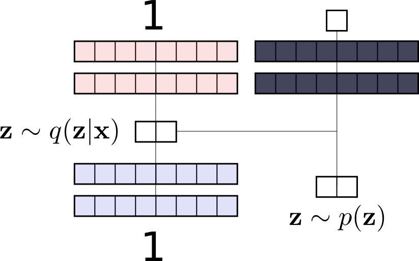
Below we demonstrate the architecture of an adversarial autoencoder. The left part of the diagram shows the encoder/decoder pair, where an input vector $\mathbf{x}$, the digit “1” in this case, is fed in as input to the encoder, transformed to the code $\mathbf{z}$ by the encoder, and then fed to the decoder that transforms it back to the original data space. On the right, a sample $\mathbf{z}$ is drawn from the prior distribution $p(\mathbf{z})$. The discriminator is optimized to separate the samples drawn from the prior distribution $p(\mathbf{z})$ from the samples drawn from the encoder distribution $q(\mathbf{z}|\mathbf{x})$.

For every minibatch, there are three important events:

1. A minibatch of input vectors is encoded and decoded by the encoder and decoder, respectively, after which both the encoder and decoder are updated based on the standard reconstruction loss.
2. A minibatch of input vectors is transformed by the encoder, after which the minibatch is concatenated with code vectors sampled from the prior distribution. The discriminator is then updated using a binary cross-entropy loss based on its ability to separate those samples generated by the encoder from those sampled from the prior distribution.
3. A minibatch of input vectors is transformed by the encoder, the source of these data points is predicted by the discriminator, and the generator (which is also the encoder) is updated using a binary cross-entropy loss based on its ability to fool the discriminator into thinking the data points came from the prior distribution.

It is interesting to note that the reconstruction loss drops fairly consistently throughout training. The adversarial losses (generative and discriminative, respectively), on the other hand, remain roughly constant after some initial fluctuation. This is the result of the adversarial training, where the discriminator’s improvement is countered by the generator’s improvement, leading to the convergence of both.

Experiments

To explore some of the properties of an adversarial autoencoder, we train it on the MNIST handwritten digit data set. The architecture we use is as described here by the author. We use two neurons in the encoder’s output layer and draw samples from a two-dimensional uniform random distribution.

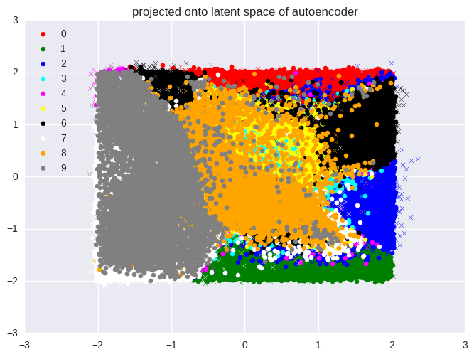
First, we show the images from the MNIST handwritten digit data set projected onto the two axes represented by the two neurons in the output of the encoder. Because we are projecting the 784-dimensional input vectors to 2-dimensional vectors, there is a lot of overlap between the classes. We clearly see, however, that practically all the data points from the training set (indicated by circles) lie within the bounds of the prior distribution. Note that some of the points from the test set (indicated by crosses) lie outside this region.

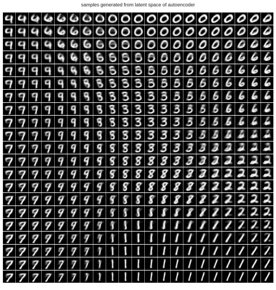
Next, we traverse the two axes of our prior distribution, sampling points from a regularly-spaced grid. For each sample, we use the decoder to generate a sample in the original data space. Note how the generated digits in each region correspond to the mapped regions of digits in the space represented by the encoder’s output.

Summary and Further Reading

We briefly discussed autoencoders and how they can be used as generative models, and then continued to describe how we can use adversarial training to impose constraints on the output distribution of the encoder. Finally, we demonstrate the ten digit classes of MNIST projected onto the encoder’s output distribution, and then traverse this space to generate realistic images in the original data space.

Those interested in further reading might want to take a look at the following links:

1. A discussion by the author on /r/machinelearning. This provides a detailed guide to implementing an adversarial autoencoder and was used extensively in my own implementation.
2. A similar post describing generative adversarial autoencoders.
3. Another implementation of an adversarial autoencoder.
4. A related paper, Deep Convolutional Generative Adversarial Networks, and the available source code.

Quantifying Uncertainty in Neural Networks

As part of my research on applying deep learning to problems in computer vision, I am trying to help plankton researchers accelerate the annotation of large data sets. In terms of the actual classification of plankton images, excellent progress has been made recently, largely thanks to the popular 2015 Kaggle National Data Science Bowl. In this competition, the goal was to predict the probability distribution function over 121 different classes of plankton, given a grayscale image containing a single plankton organism. The winning team’s solution is of particular interest, and the code is available on GitHub.

While this progress is encouraging, there are challenges that arise when using deep convolutional neural networks to annotate plankton data sets in practice. In particular, unlike in most data science competitions, the plankton species that researchers wish to label are not fixed. Even in a single lake, the relevant species may change as they are influenced by seasonal and environmental changes. Additionally, because of the difficulties involved in collecting high-quality images of plankton, a large training set is often unavailable.

For the reasons given above, for any system to be practically useful, it has to

1. recognize when an image presented for classification contains a species that was absent during training,

2. acquire the labels for the new class from the user, and

3. extend its classification capabilities to include this new class.

In this post, we consider the first point above, i.e., how we can quantify the uncertainty in a deep convolutional neural network. A brief overview with links to the relevant sections is given below.

1. Background: why interpreting softmax output as confidence scores is insufficient.
2. Bayesian Neural Networks: we look at a recent blog post by Yarin Gal that attempts to discover What My Deep Model Doesn’t Know…
3. Experiments: we attempt to quantify uncertainty in a model trained on CIFAR-10.
4. Code: all the code is available on GitHub.

Background

Although it may be tempting to interpret the values given by the final softmax layer of a convolutional neural network as confidence scores, we need to be careful not to read too much into this. For example, consider that recent work on adversarial examples has shown that imperceptible perturbations to a real image can change a deep network’s softmax output to arbitrary values. This is especially important to keep in mind when we are dealing with images from classes that were not present during training. In Deep Neural Networks are Easily Fooled: High Confidence Predictions for Unrecognizable Images, the authors explain how the region corresponding to a particular class may be much larger than the space in that region occupied by training examples from that class. The result of this is that an image may lie within the region assigned to a class and so be classified with a large peak in the softmax output, while still being far from images that occur naturally in that class in the training set.

Bayesian Neural Networks

In an excellent blog post, Yarin Gal explains how we can use dropout in a deep convolutional neural network to get uncertainty information from the model’s predictions. In a Bayesian neural network, instead of having fixed weights, each weight is drawn from some distribution. By applying dropout to all the weight layers in a neural network, we are essentially drawing each weight from a Bernoulli distribution. In practice, this mean that we can sample from the distribution by running several forward passes through the network. This is referred to as Monte Carlo dropout.

Experiments

Quantifying the uncertainty in a deep convolutional neural network’s predictions as described in the blog post mentioned above would allow us to find images for which the network is unsure of its prediction. Ideally, when given a new unlabeled data set, we could use this to find images that belong to classes that were not present during training.

To investigate this, we train a deep convolutional neural network similar to the one used in Bayesian Convolutional Neural Networks with Bernoulli Approximate Variational Inference and as described on GitHub. The goal was to train this network on the ten classes of CIFAR-10, and then evaluate the certainty of its predictions on classes from CIFAR-100 that are not present in CIFAR-10.

We train the model on the 50000 training images and used the 10000 test images provided in CIFAR-10 for validation. All parameters are the same as in the implementation provided with the paper, namely a batch size of 128, weight decay of 0.0005, and dropout applied in all layers with $p = 0.5$. 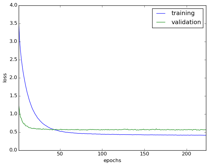The learning rate is initially set to $l = 0.01$, and is updated according to $l_{i+1} = l_{i} (1 + \gamma i)^{-p}$, with $\gamma = 0.0001$ and $p = 0.75$, after the $i$th weight update. The learning curve is shown below. The best validation loss is 0.547969 and the corresponding training loss is 0.454744.

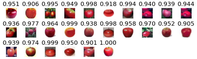
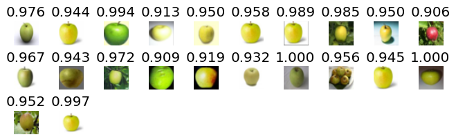
Now that we have a deep convolutional network trained on the ten classes of CIFAR-10, we present images from the apple class from CIFAR-100 to the network. We run $T=50$ stochastic forward passes through the network and take the predictive mean of the softmax output. The results, while a little discouraging, are amusing. It seems that the network is very happy to classify red apples as automobiles, and green apples as frogs with low uncertainty. Below we show apples that were classified as automobiles with $p > 0.9$, and then similarly for frogs. The number above each image is the maximum of the softmax output, computed as the mean of the 50 stochastic forward passes.

Code

All of the code used in the above experiment is available on GitHub. The non-standard dependencies are Lasagne, Theano, OpenCV (for image I/O), and Matplotlib.

Discussion

It is clear that the convolutional neural network has trouble with images that appear at least somewhat visually similar to images from classes that it saw during training. Why these misclassifications are made with low uncertainty requires further investigation. Some possibilities are mentioned below.

1. With only ten classes in CIFAR-10, it is possible that the network does not need to learn highly discriminative features to separate the classes, thereby causing the appearance of these features in another class to lead to a high-confidence output.

2. The saturating softmax output leads to the same output for two distinct classes (one present and one absent during training), even if the input to the softmax is very different for the two classes.

3. The implementation of a Bayesian neural network with Monte Carlo dropout is too crude of an approximation to accurately capture the uncertainty information when dealing with image data.

Conclusion

To build a tool that can be used by plankton researchers to perform rapid annotation of large plankton data sets, we need to quantify the uncertainty in a deep learning model’s predictions to find images from species that were not present during training. We can capture this uncertainty information with a Bayesian neural network, where dropout is used in all weight layers to represent weights drawn from a Bernoulli distribution. A quick experiment to classify a class from CIFAR-100 using a model trained only on the classes from CIFAR-10 shows that this is not trivial to achieve in practice.

Hopefully we shall be able to shed some light on the situation and address some of these problems as the topic of modeling uncertainty in deep convolutional neural networks is explored more in the literature.